Chapter 6 QIIME 2
Qiime 2 (Quantitative Insights Into Microbial Ecology 2) is a powerful, open-source bioinformatics platform designed for performing microbiome analysis from raw DNA sequencing data. It provides tools for the analysis and interpretation of high-throughput community sequencing data, facilitating tasks such as quality control, taxonomic classification, diversity analysis, and visualization. Qiime 2 supports a modular plugin system, enabling users to integrate various analytical methods and customize workflows, making it an essential tool for researchers studying microbial ecology, diversity, and function.
6.1 Use QIIME 2
Qiime 2 is already installed in the Lab Group Conda environment. To use it, follow these steps:
- Activate Conda: Run the following command to activate Conda:
- Activate the Qiime 2 Environment: Activate the Qiime 2 environment by running:
- Check the Version: Run the following command to check if Qiime 2 is installed and to see the version number:
6.2 Available Qiime 2 Databases
A pre-trained classifier database for Qiime 2 is available in the Group Directory. This database can be found under the following directory:
/mnt/vstor/SOM_PQHS_LXZ716/Reference
The available database includes:
QIIME2_Pre-trained_Classifier: A pre-trained classifier for taxonomic classification of microbial sequences, optimized for use with Qiime 2.
6.3 Example for Jax.IU.Pitt Microbiome Pilot Study
6.3.1 Importing Data
Fastq Manifest Formats
When importing data, we use the “Fastq manifest” format. This method is suitable for data that do not fit the common multiplexed or demultiplexed formats (e.g., EMP or Casava). To import your data manually, you will need to create a manifest file and use the qiime tools import command.
Format Description
First, you’ll create a text file called a “manifest file”, which maps sample identifiers to fastq.gz or fastq absolute filepaths that contain sequence and quality data for the sample (i.e., these are FASTQ files). The manifest file also indicates the direction of the reads in each fastq.gz or fastq file. The manifest file is designed to be a simple format that doesn’t put restrictions on the naming of the demultiplexed fastq.gz / fastq files.
The manifest file is a tab-separated (i.e., .tsv) text file. The first column defines the Sample ID, while the second (and optional third) column defines the absolute filepath to the forward (and optional reverse) reads. The fastq.gz absolute filepaths may contain environment variables (e.g., $HOME or $PWD).
Example Manifest File for Paired-End Reads
Here is an example of a manifest file for paired-end read data:
sample-id    forward-absolute-filepath                    reverse-absolute-filepath
288593663    /mnt/vstor/SOM_PQHS_LXZ716/MicroB2/288593663_R1.fastq.gz    /mnt/vstor/SOM_PQHS_LXZ716/MicroB2/288593663_R2.fastq.gz
288601191    /mnt/vstor/SOM_PQHS_LXZ716/MicroB2/288601191_R1.fastq.gz    /mnt/vstor/SOM_PQHS_LXZ716/MicroB2/288601191_R2.fastq.gz
288605432    /mnt/vstor/SOM_PQHS_LXZ716/MicroB2/288605432_R1.fastq.gz    /mnt/vstor/SOM_PQHS_LXZ716/MicroB2/288605432_R2.fastq.gz
288613647    /mnt/vstor/SOM_PQHS_LXZ716/MicroB2/288613647_R1.fastq.gz    /mnt/vstor/SOM_PQHS_LXZ716/MicroB2/288613647_R2.fastq.gz
288625970    /mnt/vstor/SOM_PQHS_LXZ716/MicroB2/288625970_R1.fastq.gz    /mnt/vstor/SOM_PQHS_LXZ716/MicroB2/288625970_R2.fastq.gz
288638583    /mnt/vstor/SOM_PQHS_LXZ716/MicroB2/288638583_R1.fastq.gz    /mnt/vstor/SOM_PQHS_LXZ716/MicroB2/288638583_R2.fastq.gz
288638603    /mnt/vstor/SOM_PQHS_LXZ716/MicroB2/288638603_R1.fastq.gz    /mnt/vstor/SOM_PQHS_LXZ716/MicroB2/288638603_R2.fastq.gz
288658590    /mnt/vstor/SOM_PQHS_LXZ716/MicroB2/288658590_R1.fastq.gz    /mnt/vstor/SOM_PQHS_LXZ716/MicroB2/288658590_R2.fastq.gz
288662694    /mnt/vstor/SOM_PQHS_LXZ716/MicroB2/288662694_R1.fastq.gz    /mnt/vstor/SOM_PQHS_LXZ716/MicroB2/288662694_R2.fastq.gz
288696281    /mnt/vstor/SOM_PQHS_LXZ716/MicroB2/288696281_R1.fastq.gz    /mnt/vstor/SOM_PQHS_LXZ716/MicroB2/288696281_R2.fastq.gz
Importing the Data
Use the following command to import the data into QIIME 2:
qiime tools import \
  --type 'SampleData[PairedEndSequencesWithQuality]' \
  --input-path /mnt/vstor/SOM_PQHS_LXZ716/MicroB2/manifest.tsv \
  --output-path /mnt/vstor/SOM_PQHS_LXZ716/MicroB2/Analysis_QIIME2/paired-end-demux.qza \
  --input-format PairedEndFastqManifestPhred33V2
For more information on importing data and using different formats, refer to the QIIME 2 Importing Tutorial.
6.3.2 Trimming Adapters from Sequences
After importing the data, it is important to remove any adapter sequences that may be present. The trimmed sequences can often be found in the STUDY DESCRIPTION. For example, in our study, the STUDY DESCRIPTION mentions:
The primers used incorporated Illumina dual indices and sequencing adapters with the following 16S rRNA gene V1-V3 priming regions: 27F (5’ AGAGTTTGATCCTGGCTCAG) and 534R (5’ ATTACCGCGGCTGCTGG).
Use the following command to trim adapters from the paired-end sequences:
qiime cutadapt trim-paired \
  --i-demultiplexed-sequences /mnt/vstor/SOM_PQHS_LXZ716/MicroB2/Analysis_QIIME2/paired-end-demux.qza \
  --p-cores 16 \
  --p-front-f AGAGTTTGATCCTGGCTCAG \
  --p-front-r ATTACCGCGGCTGCTGG \
  --p-discard-untrimmed \
  --o-trimmed-sequences /mnt/vstor/SOM_PQHS_LXZ716/MicroB2/Analysis_QIIME2/trim-seqs.qza \
--verbose--i-demultiplexed-sequences: Input file with demultiplexed sequences.--p-cores: Number of CPU cores to use for processing.--p-front-f: Forward adapter sequence to trim.--p-front-r: Reverse adapter sequence to trim.--p-discard-untrimmed: Discard reads that do not contain the adapter sequences.--o-trimmed-sequences: Output file for the trimmed sequences.--verbose: Provides detailed output during the trimming process.
After trimming the adapters, proceed to the summarizing demultiplexed sequences step to visualize the quality of the trimmed data.
6.3.3 Summarizing Demultiplexed Sequences
Before denoising, it is important to visualize the quality of the sequencing data. This step summarizes the demultiplexed sequences and generates a visualization to help determine the optimal truncation lengths for denoising.
qiime demux summarize \
  --i-data /mnt/vstor/SOM_PQHS_LXZ716/MicroB2/Analysis_QIIME2/trim-seqs.qza \
--o-visualization /mnt/vstor/SOM_PQHS_LXZ716/MicroB2/Analysis_QIIME2/trim-seqs.qzv--i-data: Input file with demultiplexed sequences.--o-visualization: Output file for the summary visualization.
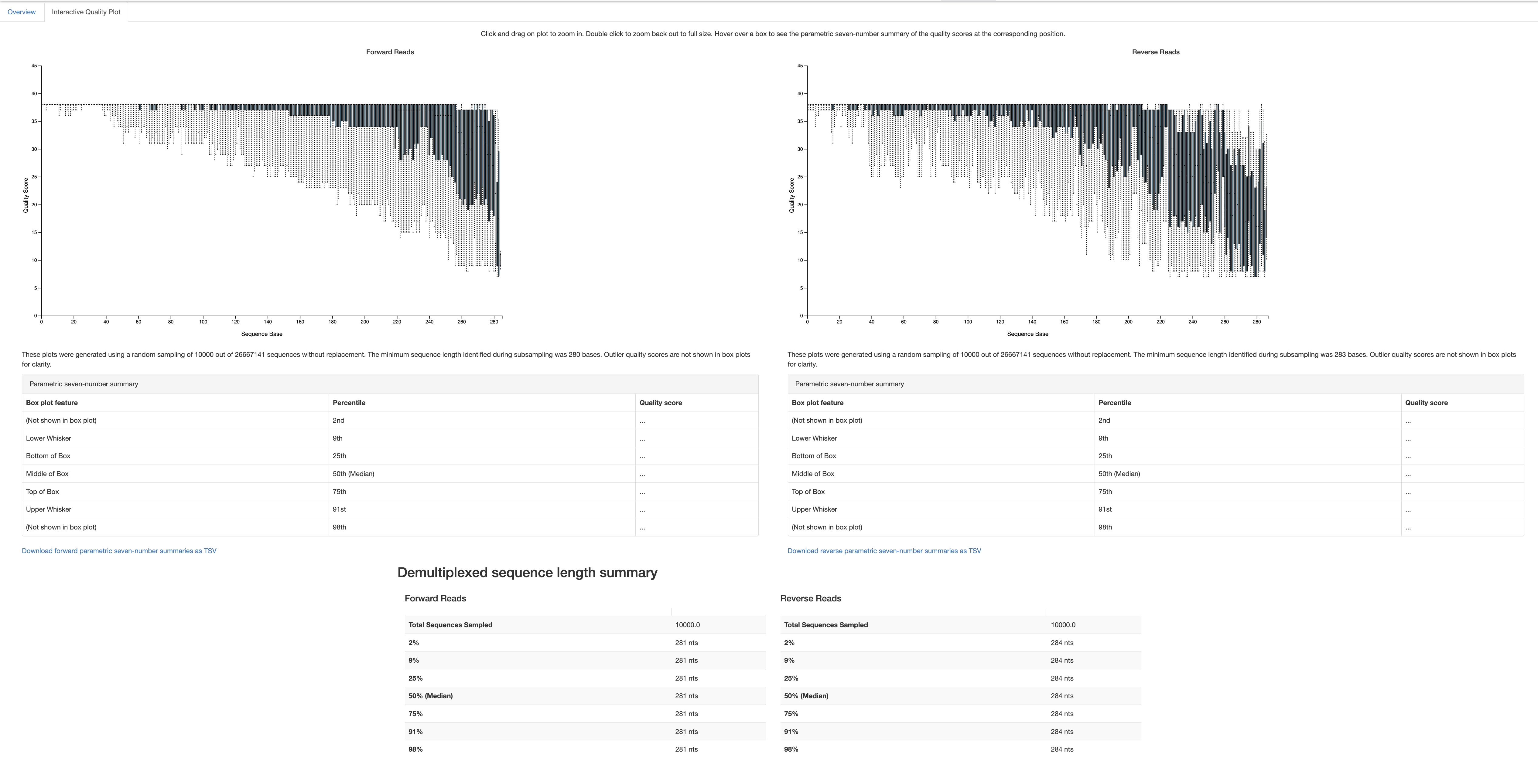
The output visualization (demux-summary.qzv) provides interactive plots of the quality scores across all sequences. This information is crucial for determining the appropriate truncation lengths (--p-trunc-len-f and --p-trunc-len-r) to use in the denoising step.
How to Choose Truncation Lengths:
- Open the Visualization:
Open the demux-summary.qzv file in QIIME 2 View QIIME 2 View.
- Inspect the Quality Plots:
Look at the interactive quality plots for the forward and reverse reads. Each plot shows the distribution of quality scores across all positions in your reads.
- Identify Quality Drop-off Points:
Identify the position in the reads where the quality scores start to drop significantly. This is usually seen as a downward trend in the quality scores towards the end of the reads. For example, if the quality scores drop below a threshold (e.g., Q25) around position 270 for the forward reads and position 260 for the reverse reads, these positions might be suitable truncation points.
- Choose Conservative Truncation Lengths:
To ensure high-quality data, choose truncation lengths that are slightly before the quality scores drop significantly. This helps to retain more high-quality bases. In this example, you might choose –p-trunc-len-f 270 for the forward reads and –p-trunc-len-r 260 for the reverse reads.
6.3.4 Denoising Sequences with DADA2
This step removes noise from the sequencing data, corrects errors, and generates a table of feature abundances (ASVs), representative sequences, and denoising statistics.
qiime dada2 denoise-paired \
  --i-demultiplexed-seqs /mnt/vstor/SOM_PQHS_LXZ716/MicroB2/Analysis_QIIME2/trim-seqs.qza \
  --p-trim-left-f 0 \
  --p-trim-left-r 0 \
  --p-trunc-len-f 270 \
  --p-trunc-len-r 260 \
  --o-table /mnt/vstor/SOM_PQHS_LXZ716/MicroB2/Analysis_QIIME2/table.qza \
  --o-representative-sequences /mnt/vstor/SOM_PQHS_LXZ716/MicroB2/Analysis_QIIME2/rep-seqs.qza \
--o-denoising-stats /mnt/vstor/SOM_PQHS_LXZ716/MicroB2/Analysis_QIIME2/denoising-stats.qza--i-demultiplexed-seqs: Input file with demultiplexed sequences.--p-trim-left-fand--p-trim-left-r: Number of bases to trim from the start of each read.--p-trunc-len-fand--p-trunc-len-r: Position at which reads are truncated due to decrease in quality.--o-table: Output file for the feature table (ASVs).--o-representative-sequences: Output file for the representative sequences.--o-denoising-stats: Output file for denoising statistics.
6.3.5 Taxonomic Classification
This step classifies the representative sequences into taxonomic groups using a pre-trained classifier.
qiime feature-classifier classify-sklearn \
  --i-classifier /mnt/vstor/SOM_PQHS_LXZ716/Reference/QIIME2_Pre-trained_Classifier/silva-138-99-nb-classifier.qza \
  --i-reads /mnt/vstor/SOM_PQHS_LXZ716/MicroB2/Analysis_QIIME2/rep-seqs.qza \
--o-classification /mnt/vstor/SOM_PQHS_LXZ716/MicroB2/Analysis_QIIME2/taxonomy.qza--i-classifier: Pre-trained classifier file.--i-reads: Input file with representative sequences.--o-classification: Output file with taxonomic classification results.
6.3.6 Metadata Visualization
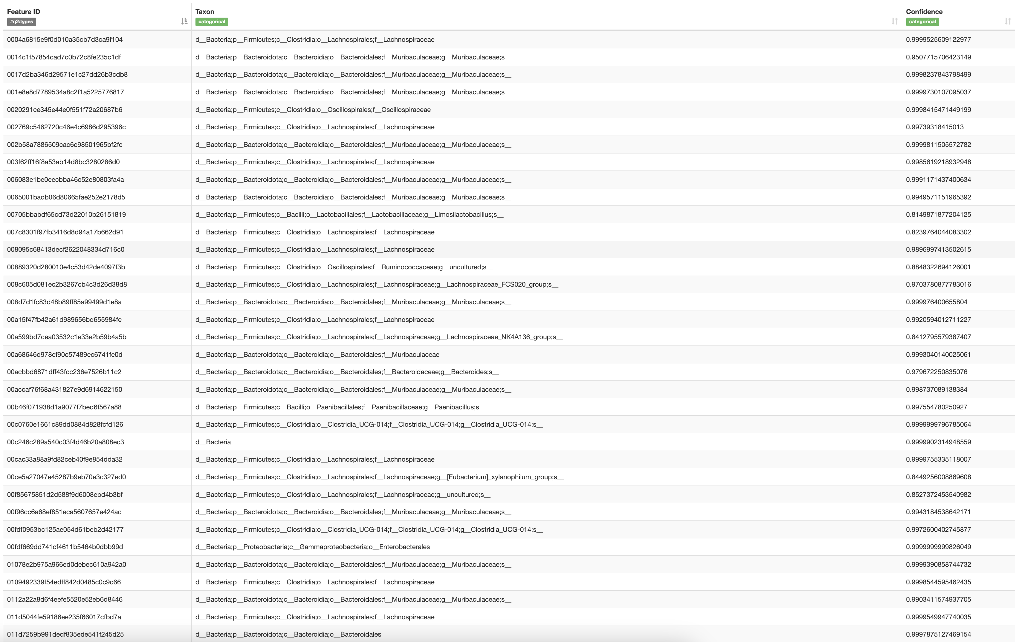
This step creates a visualization of the taxonomic classification results, allowing you to review the taxonomy assignments.
qiime metadata tabulate \
  --m-input-file /mnt/vstor/SOM_PQHS_LXZ716/MicroB2/Analysis_QIIME2/taxonomy.qza \
--o-visualization /mnt/vstor/SOM_PQHS_LXZ716/MicroB2/Analysis_QIIME2/taxonomy.qzv--m-input-file: Input file with metadata to be visualized.--o-visualization: Output file for the visualization.
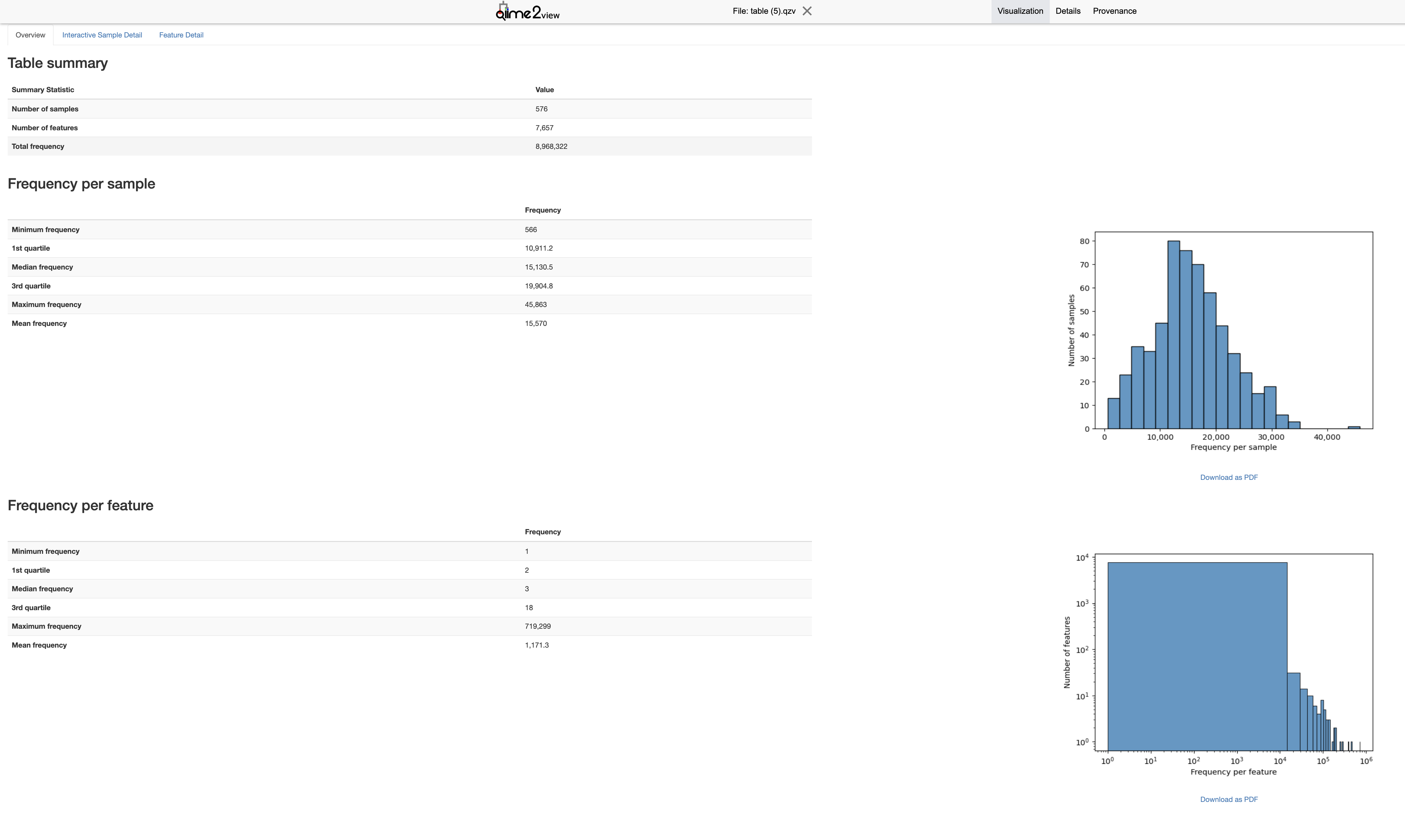
6.3.7 Feature Table Summary
This step summarizes the feature table, providing an overview of feature counts per sample and other summary statistics.
qiime feature-table summarize \
  --i-table /mnt/vstor/SOM_PQHS_LXZ716/MicroB2/Analysis_QIIME2/table.qza \
  --o-visualization /mnt/vstor/SOM_PQHS_LXZ716/MicroB2/Analysis_QIIME2/table.qzv \
--m-sample-metadata-file /mnt/vstor/SOM_PQHS_LXZ716/MicroB2/processed_metadata.tsv--i-table: Input feature table file.--o-visualization: Output file for the summary visualization.--m-sample-metadata-file: Metadata file associated with the samples.
6.3.8 Phylogenetic Tree Construction
This step aligns the sequences, masks the alignment to remove highly variable positions, and constructs a phylogenetic tree for diversity analyses.
qiime phylogeny align-to-tree-mafft-fasttree \
  --i-sequences /mnt/vstor/SOM_PQHS_LXZ716/MicroB2/Analysis_QIIME2/rep-seqs.qza \
  --o-alignment /mnt/vstor/SOM_PQHS_LXZ716/MicroB2/Analysis_QIIME2/aligned-rep-seqs.qza \
  --o-masked-alignment /mnt/vstor/SOM_PQHS_LXZ716/MicroB2/Analysis_QIIME2/masked-aligned-rep-seqs.qza \
  --o-tree /mnt/vstor/SOM_PQHS_LXZ716/MicroB2/Analysis_QIIME2/unrooted-tree.qza \
--o-rooted-tree /mnt/vstor/SOM_PQHS_LXZ716/MicroB2/Analysis_QIIME2/rooted-tree.qza--i-sequences: Input file with representative sequences.--o-alignment: Output file for aligned sequences.--o-masked-alignment: Output file for masked alignment.--o-tree: Output file for unrooted phylogenetic tree.--o-rooted-tree: Output file for rooted phylogenetic tree.
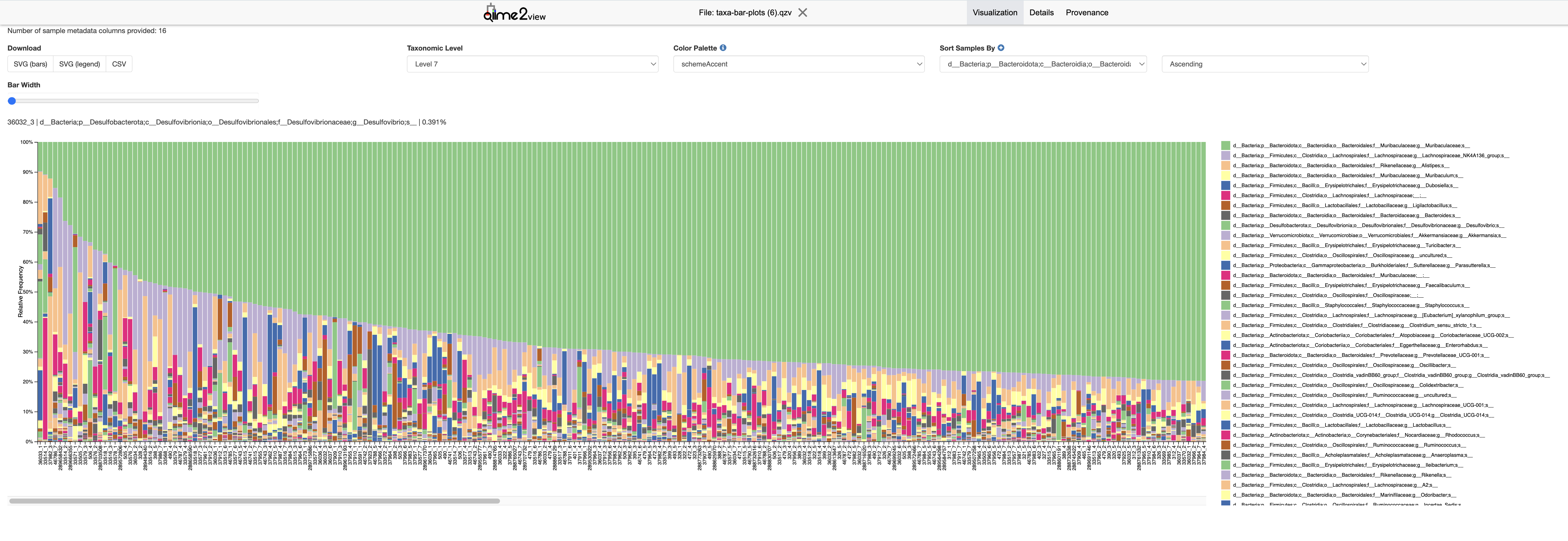
6.3.9 Taxa Bar Plot Visualization
This step creates a bar plot to visualize the taxonomic composition of the samples, providing insights into the relative abundance of different taxa.
qiime taxa barplot \
  --i-table /mnt/vstor/SOM_PQHS_LXZ716/MicroB2/Analysis_QIIME2/table.qza \
  --i-taxonomy /mnt/vstor/SOM_PQHS_LXZ716/MicroB2/Analysis_QIIME2/taxonomy.qza \
  --m-metadata-file /mnt/vstor/SOM_PQHS_LXZ716/MicroB2/processed_metadata.tsv \
--o-visualization /mnt/vstor/SOM_PQHS_LXZ716/MicroB2/Analysis_QIIME2/taxa-bar-plots.qzv--i-table: Input feature table file.--i-taxonomy: Input file with taxonomic classification.--m-metadata-file: Metadata file associated with the samples.--o-visualization: Output file for the bar plot visualization.
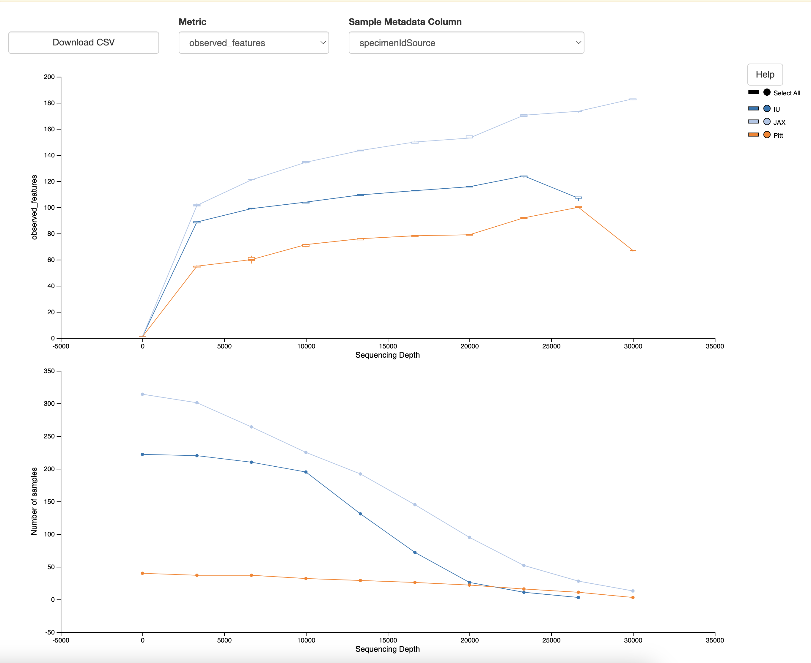
6.3.10 Alpha Rarefaction Analysis
Alpha rarefaction analysis helps to understand the diversity within a sample. This step generates a rarefaction curve, which is useful for assessing the sampling depth required to capture the diversity within each sample.
qiime diversity alpha-rarefaction \
  --i-table /mnt/vstor/SOM_PQHS_LXZ716/MicroB2/Analysis_QIIME2/table.qza \
  --i-phylogeny /mnt/vstor/SOM_PQHS_LXZ716/MicroB2/Analysis_QIIME2/rooted-tree.qza \
  --p-max-depth 30000 \
  --m-metadata-file /mnt/vstor/SOM_PQHS_LXZ716/MicroB2/processed_metadata.tsv \
--o-visualization /mnt/vstor/SOM_PQHS_LXZ716/MicroB2/Analysis_QIIME2/alpha-rarefaction.qzv--i-table: Input feature table file.--i-phylogeny: Input phylogenetic tree file.--p-max-depth: Maximum rarefaction depth.--m-metadata-file: Metadata file associated with the samples.--o-visualization: Output file for the rarefaction visualization.
Choosing --p-max-depth:
The --p-max-depth parameter specifies the maximum sequencing depth for rarefaction. To choose an appropriate value, follow these steps:
- Visualize Sequence Depth Distribution:
- Before setting
--p-max-depth, examine the sequencing depth distribution using thetable.qzvfile. This file can be generated with the following command:
qiime feature-table summarize \
  --i-table /mnt/vstor/SOM_PQHS_LXZ716/MicroB2/Analysis_QIIME2/table.qza \
  --o-visualization /mnt/vstor/SOM_PQHS_LXZ716/MicroB2/Analysis_QIIME2/table.qzv \
--m-sample-metadata-file /mnt/vstor/SOM_PQHS_LXZ716/MicroB2/processed_metadata.tsv- Open the resulting
table.qzvfile in QIIME 2 View to explore the sequencing depth distribution.
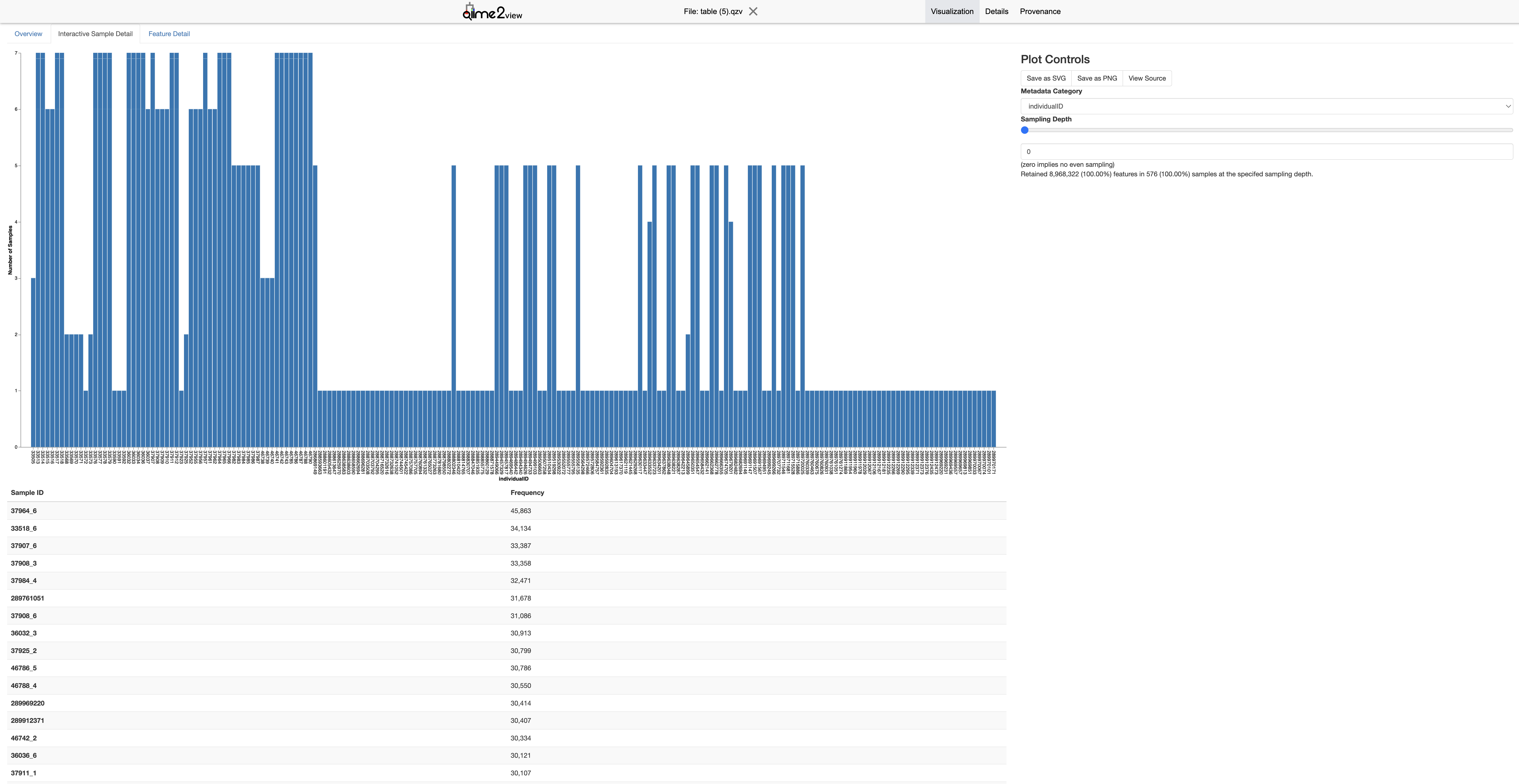
- Determine an Appropriate Depth:
- Look at the
"Interactive Sample Detail"and"Frequency per sample"plot in thetable.qzvvisualization. Select a --p-max-depthvalue that includes the majority of your samples. This helps ensure that a sufficient number of samples are included in the analysis. - Avoid setting the depth too high, as this may exclude many samples with lower sequencing depth. Conversely, setting it too low may not fully capture the diversity within each sample.
- Example:
- If the frequency plot shows that most samples have around 20,000 sequences, you might choose a –p-max-depth of 20,000 or slightly lower (e.g., 15,000) to include as many samples as possible while still capturing the diversity.
The resulting visualization (alpha-rarefaction.qzv) allows you to explore the alpha diversity metrics at different sampling depths and helps to determine the adequate sequencing depth for your samples.
6.3.11 Core Metrics Phylogenetic Analysis
Core metrics phylogenetic analysis computes a range of diversity metrics, including both alpha and beta diversity metrics. The --p-sampling-depth parameter should be chosen based on the results of the alpha rarefaction analysis.
qiime diversity core-metrics-phylogenetic \
  --i-phylogeny /mnt/vstor/SOM_PQHS_LXZ716/MicroB2/Analysis_QIIME2/rooted-tree.qza \
  --i-table /mnt/vstor/SOM_PQHS_LXZ716/MicroB2/Analysis_QIIME2/table.qza \
  --p-sampling-depth 4000 \
  --m-metadata-file /mnt/vstor/SOM_PQHS_LXZ716/MicroB2/processed_metadata.tsv \
  --o-rarefied-table /mnt/vstor/SOM_PQHS_LXZ716/MicroB2/Analysis_QIIME2/rarefied-table.qza \
  --o-observed-features-vector /mnt/vstor/SOM_PQHS_LXZ716/MicroB2/Analysis_QIIME2/observed-features.qza \
  --o-shannon-vector /mnt/vstor/SOM_PQHS_LXZ716/MicroB2/Analysis_QIIME2/shannon.qza \
  --o-evenness-vector /mnt/vstor/SOM_PQHS_LXZ716/MicroB2/Analysis_QIIME2/evenness.qza \
  --o-faith-pd-vector /mnt/vstor/SOM_PQHS_LXZ716/MicroB2/Analysis_QIIME2/faith-pd.qza \
  --o-unweighted-unifrac-distance-matrix /mnt/vstor/SOM_PQHS_LXZ716/MicroB2/Analysis_QIIME2/unweighted-unifrac-distance-matrix.qza \
  --o-weighted-unifrac-distance-matrix /mnt/vstor/SOM_PQHS_LXZ716/MicroB2/Analysis_QIIME2/weighted-unifrac-distance-matrix.qza \
  --o-jaccard-distance-matrix /mnt/vstor/SOM_PQHS_LXZ716/MicroB2/Analysis_QIIME2/jaccard-distance-matrix.qza \
  --o-bray-curtis-distance-matrix /mnt/vstor/SOM_PQHS_LXZ716/MicroB2/Analysis_QIIME2/bray-curtis-distance-matrix.qza \
  --o-unweighted-unifrac-pcoa-results /mnt/vstor/SOM_PQHS_LXZ716/MicroB2/Analysis_QIIME2/unweighted-unifrac-pcoa-results.qza \
  --o-weighted-unifrac-pcoa-results /mnt/vstor/SOM_PQHS_LXZ716/MicroB2/Analysis_QIIME2/weighted-unifrac-pcoa-results.qza \
  --o-jaccard-pcoa-results /mnt/vstor/SOM_PQHS_LXZ716/MicroB2/Analysis_QIIME2/jaccard-pcoa-results.qza \
  --o-bray-curtis-pcoa-results /mnt/vstor/SOM_PQHS_LXZ716/MicroB2/Analysis_QIIME2/bray-curtis-pcoa-results.qza \
  --o-unweighted-unifrac-emperor /mnt/vstor/SOM_PQHS_LXZ716/MicroB2/Analysis_QIIME2/unweighted-unifrac-emperor.qzv \
  --o-weighted-unifrac-emperor /mnt/vstor/SOM_PQHS_LXZ716/MicroB2/Analysis_QIIME2/weighted-unifrac-emperor.qzv \
  --o-jaccard-emperor /mnt/vstor/SOM_PQHS_LXZ716/MicroB2/Analysis_QIIME2/jaccard-emperor.qzv \
--o-bray-curtis-emperor /mnt/vstor/SOM_PQHS_LXZ716/MicroB2/Analysis_QIIME2/bray-curtis-emperor.qzv--i-phylogeny: Input phylogenetic tree file.--i-table: Input feature table file.--p-sampling-depth: Depth at which to subsample the feature table for diversity metrics.--m-metadata-file: Metadata file associated with the samples.--o-rarefied-table: Output rarefied feature table, used for subsequent diversity analyses.--o-observed-features-vector: Output vector of observed features, representing the number of unique features (e.g., species) observed in each sample.--o-shannon-vector: Output vector of Shannon diversity index, a measure of the richness and evenness of species in a community.--o-evenness-vector: Output vector of Pielou’s evenness, indicating how evenly the individuals are distributed across the different species present.--o-faith-pd-vector: Output vector of Faith’s Phylogenetic Diversity, a measure of diversity that considers the phylogenetic relationships between species.--o-unweighted-unifrac-distance-matrix: Output unweighted UniFrac distance matrix, a measure of beta diversity that considers the presence/absence of species and their phylogenetic relationships.--o-weighted-unifrac-distance-matrix: Output weighted UniFrac distance matrix, similar to unweighted UniFrac but also considering the relative abundance of species.--o-jaccard-distance-matrix: Output Jaccard distance matrix, a measure of beta diversity based on the presence/absence of species.--o-bray-curtis-distance-matrix: Output Bray-Curtis distance matrix, a measure of beta diversity that considers the relative abundance of species.--o-unweighted-unifrac-pcoa-results: Output PCoA results for unweighted UniFrac, used for visualizing the beta diversity.--o-weighted-unifrac-pcoa-results: Output PCoA results for weighted UniFrac, used for visualizing the beta diversity.--o-jaccard-pcoa-results: Output PCoA results for Jaccard distance, used for visualizing the beta diversity.--o-bray-curtis-pcoa-results: Output PCoA results for Bray-Curtis distance, used for visualizing the beta diversity.--o-unweighted-unifrac-emperor: Output Emperor visualization for unweighted UniFrac, an interactive visualization tool.--o-weighted-unifrac-emperor: Output Emperor visualization for weighted UniFrac, an interactive visualization tool.--o-jaccard-emperor: Output Emperor visualization for Jaccard distance, an interactive visualization tool.--o-bray-curtis-emperor: Output Emperor visualization for Bray-Curtis distance, an interactive visualization tool.
Choosing –p-sampling-depth:
The --p-sampling-depth parameter should be chosen based on the results of the alpha rarefaction analysis. In the alpha rarefaction visualization (alpha-rarefaction.qzv), look at the sequencing depth at which the observed features plateau for most samples. This depth ensures that the diversity metrics are calculated with an adequate number of sequences without excluding too many samples. For example, if the observed features plateau around 4,000 sequences, you might set --p-sampling-depth to 4,000.